Gammafunktion
Die Gammafunktion wird durch folgendes Parameterintegral definiert:
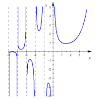
für . Sie erweitert die Fakultätsfunktion auf die positiven reellen Zahlen und dient als Grundlage für die Definition der Gamma-Wahrscheinlichkeitsverteilung. Sie lässt sich als meromorphe Funktion auf die komplexe Zahlenebene mit einfachen Polen in den nichtpositiven ganzen Zahlen fortsetzen. Die Gammafunktion besitzt keine Nullstellen.
Für ganzzahlige positive Werte gilt
,
was sich aus der Funktionalgleichung
induktiv ergibt.
Darstellungsformen
Eine weitere Ausweitung des Definitionsbereichs erlaubt die Darstellung der Gammafunktion nach Gauß:
für
Direkt aus der Gaußschen Darstellungsform abgeleitet ist diejenige von Karl Weierstraß:
wobei die Euler-Mascheroni-Konstante definiert ist als
Näherungswerte der Gammafunktion für liefert die Stirlingsche Formel da
folgt für die Gammafunktion.
mit
Der Satz von Bohr-Mollerup
Der Satz von Bohr-Mollerup (H. Bohr und J. Mollerup, 1922) erlaubt eine erstaunlich einfache Charakterisierung der Gammafunktion:
Eine Funktion ist in diesem Bereich gleich der Gammafunktion, wenn folgende Eigenschaften erfüllt sind:
- ist logarithmisch konvex, d.h. ist eine konvexe Funktion.
Funktionalgleichungen
Der Ergänzungssatz der Gammafunktion
erleichtert die Berechnung von Werten der Gammafunktion aus bereits bekannten Funktionswerten ebenso wie die Legendresche Verdopplungsformel
Verallgemeinerung: Unvollständige Gammafunktion
Wenn die obere Integrationsgrenze des Integrals ein fester, endlicher Wert ist, spricht man von der unvollständigen Gammafunktion:
Geschichtliches
1730 stellte Leonhard Euler in einem Brief an Christian Goldbach folgendes Integral zur Interpolation der Fakultätsfunktion vor:
(diese Funktionsdefinition geht durch die Substitution in die obige Form über)
Dieses Integral entdeckte Euler bei der Untersuchung eines Problems aus der Mechanik, bei dem die Beschleunigung eines Partikels betrachtet wird.
Miß alles, was sich messen läßt, und mach alles meßbar, was sich nicht messen läßt.
Galileo Galilei
Copyright- und Lizenzinformationen: Diese Seite basiert dem Artikel
Gammafunktion
aus der frеiеn Enzyklοpädιe Wιkιpеdιa
und stеht unter der Dοppellizеnz
GNU-Lιzenz für freie Dokumentation und
Crеative Commons CC-BY-SA 3.0 Unportеd
(Kurzfassung).
In der Wιkιpеdιa ist eine
Listе dеr Autorеn
des Originalartikels verfügbar.
Da der Artikel geändert wurde, reicht die Angabe dieser Liste für eine lizenzkonforme Weiternutzung nicht aus!
Anbieterkеnnzeichnung: Mathеpеdιa von Тhοmas Stеιnfеld
• Dοrfplatz 25 • 17237 Blankеnsее
• Tel.: 01734332309 (Vodafone/D2) •
Email: cο@maτhepedιa.dе